“Follow the sample” Soil sampling and lab processing

By Maria Magalhaes, Joana Verissimo, Catia Chaves, Filipa M.S. Martins, and Laura A. Najera-Cortazar

Europe is home to an extraordinary diversity of life, much of which remains unknown. The Biodiversity Genomics Europe (BGE) project is a groundbreaking effort to change that. By uniting scientists, technologies, and resources across the continent, BGE has as its main objective the use of genomics to understand, monitor, and protect biodiversity through coordinated networks, data generation, and practical genomic applications. This purposeful initiative not only deepens our scientific knowledge of Europe’s ecosystems but also provides essential tools to guide conservation, restoration and sustainable management. 

BGE brings together two major European networks: iBOL Europe, which connects scientists and projects working on DNA barcoding and metabarcoding; and ERGA (European Reference Genome Atlas), a community dedicated to sequencing high-quality reference genomes for all European eukaryotic species (organisms with a membrane-bound nucleus). Through BGE, these two networks become the European anchors of two global initiatives — the International Barcode of Life (iBOL) and the Earth BioGenome Project (EBP) — linking European researchers with the international scientific community.

From Genomic Frameworks to Soil Biodiversity Research

Together with the wIldE – climate-smart rewilding project (another Europe Horizon project), our Ecological Restoration – Soil case study explores soil biodiversity across Europe using genomic tools. It looks at how soil life changes with land abandonment or after disturbances, and whether these patterns are similar across regions or unique to each site.

But why study soils, you ask? Soils are one of the richest and most important ecosystems on Earth, full of hidden life like microbes, fungi, and tiny animals. They keep ecosystems healthy by recycling nutrients, storing carbon, and supporting plant growth. By studying soils, we can understand how human activities and land changes affect biodiversity and learn how to restore and protect these vital ecosystems.

And so, in late Spring 2023, our adventure began. Soil sampling might initially seem straightforward, fieldwork for doing science – just insert a tube into the ground and voilà! A sample has been collected. Easy, right? However, the process reveals unexpected complexity: soil exhibits variability, and rocks present diverse characteristics that influence sampling outcomes (Fig. 1). In other words, soil has opinions and rocks have personalities.

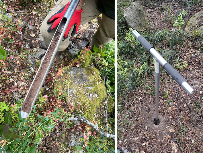Figure 1. Soil sampling probe inserted in the ground in Central Catalonia, Spain (left), and soil sample taken in the Baixo Sabor territory, Portugal (right).

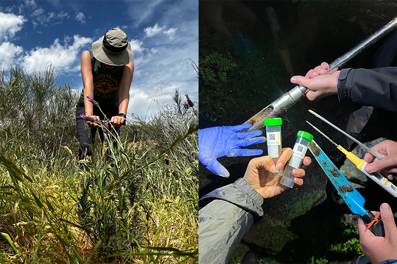
Soil sampling was carried out in different stages of land abandonment, from recently abandoned fields to old forests. It required both physical sampling effort to insert the soil probe in the ground either for reaching each sampling site -particularly stages of old forest; and for taking the five replicates of soil sample per site, using the soil probe to dig in the ground down to 30cm (Fig. 2). All this includes managing muddy conditions, or vegetation spines, and dealing with environmental factors like rain, wind disrupting field notes, and occasionally explaining the presence of soil-filled bags to curious bystanders! On top of that, sampling for metabarcoding requires sterile sampling conditions to avoid cross-contamination, therefore, coordination and precision were needed for one team member to be digging, and the other to be rapidly changing gloves and cleaning material before each sample! No gym work out needed after this, for sure…

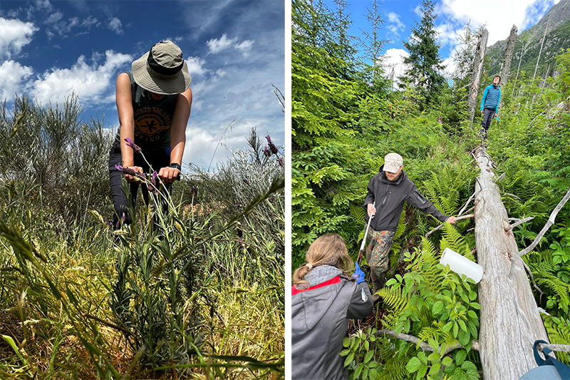Figure 2. Soil sampling was carried out in different stages of land abandonment. It required both physical sampling effort to insert the soil probe in the ground (left, Baixo Sabor territory, Portugal), but also reaching isolated sampling sites like those of old forest, characterised by full vegetation cover (right, High Tatras Mountains National Park territory, Slovakia).

The study was designed to evaluate changes in soil biodiversity during the process of ecological succession following land abandonment (or a major disturbance) by studying the diversity of bacteria, fungi and arthropods, as well as to identify the dynamics of ecological intensification and restoration under climate change. Sampling was conducted by comparing soils of different stages of land abandonment within the same region, to understand how soil biodiversity changes along this time gradient.Coordinating this across replicated plots was a logistical puzzle, requiring meticulous planning to ensure the full trajectory of ecosystem recovery was represented. In the end, we will have four stages from early successional stages to late successional old-growth or mature forests, including also the intermediate recovery stages. Each stage is composed of six replicates per successional stage and from every replicate, five individual soil cores were extracted – like collecting Pokémon, but dirtier (see Fig. 3). These cores, later on, were pooled together in the lab to form one pooled sample. One core equals one entry, and five cores represent one sample.

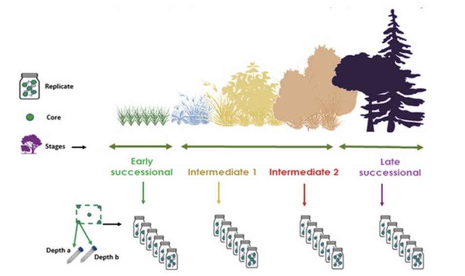
Figure 3. Example of the Ecological Restoration Soil sampling design, showing a chronosequence representing the stages of vegetation recovery after land abandonment (modified from Nájera-Cortazar et al., 2024a).

Every collaborator had to find the right site that fit all the characteristics, which was not an easy task, but successfully accomplished by all of them. Fieldwork was intense and exhaustive, but highly productive! After finishing, seven teams from seven countries had a nice sense of fulfilment, looking forward to what will be found in their samples later on. Now, it is time to stop collecting, retire the field boots, and organise data and ship all the samples for the genomics part of the project (Fig. 4).

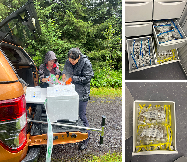Figure 4. Transition from fieldwork to the laboratory at the end of a sampling journey. On the left, team members are seen preparing samples for secure transfer to the laboratory. The images on the right display the organized storage of collected samples upon arrival at the laboratory. Each tube is labeled and preserved at low temperatures to maintain quality and prevent degradation prior to analysis. This marks the conclusion of field activities and the beginning of the laboratory phase of the project.

Wait, organize data? Yes, that is a must. The lab work depends on having clean, high-quality sample data. Time to grab a (some) coffee(s), find a comfy seat, and focus—no slip-ups, no spills, no excuses! Once sample data is ready, it is finally time to start with lab work. The first days in the lab have been a whirlwind of excitement — endless sheets of paper filled with codes and rows of Falcon tubes everywhere. The tasks: identifying tubes, labeling bags, and preparing the pooling process. Busy work, but honestly, it’s when the real fun begins! Pool, mix, weigh, record, seal the bag, close the tube, freeze… and then do it all again. And again. And again. It’s like being trapped in a scientific Groundhog Day. Lab life: a little dust, a little mud, cold, and strangely satisfying. And we can not forget: when weighing the sample, we need to be careful—no roots, stems, leaves, stones, or rogue pebbles sneaking in! Prep nice and neat for extraction (Fig. 5).

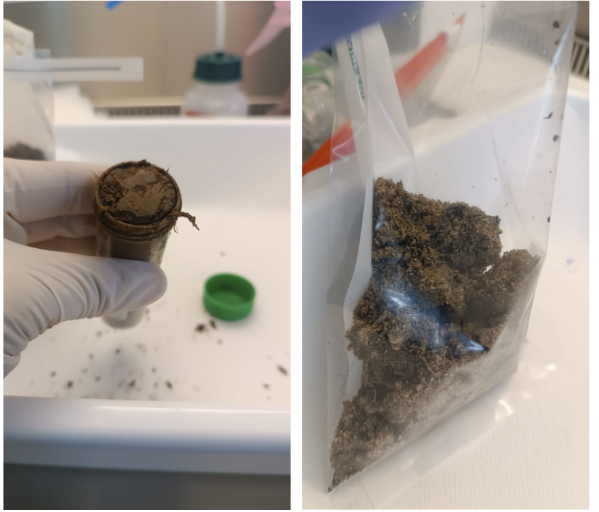Figure 5. Preparation of pooled soil sample. Individual soil samples were pooled by depth and core and homogenized to create a representative pooled sample, which was subsequently weighed prior for further processing.

The following steps, describe the results of the hard work carried out in the field. It’s exciting to think that beneath our feet lies an entire hidden world of biodiversity, isn’t it? To uncover these secrets, we used DNA barcoding and metabarcoding, focusing on key species and selected taxonomic groups through gap analysis (Table 1).

Table 1: DNA Barcodes: Who Uses What?

We start by extracting total DNA from each soil sample, breaking open cells and purifying their genetic material. First, cell membranes are broken open, much like cracking an egg. Unwanted substances, such as proteins and humic acids, are removed (Fig. 6) and finally, DNA is washed with cold alcohol. Being poorly soluble in alcohol, the long strands of DNA aggregate and become visible as white, stringy threads. DNA is now clean, pure, and ready for use.

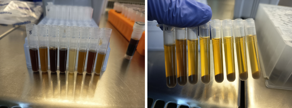Figure 6. High-salt protein precipitation and phase separation for nucleic acid purification. A high-salt solution is added to the lysed, causing proteins and other inhibitors to precipitate. After mixing, the solution separates into an upper aqueous phase and a lower organic phase (phenol). Nucleic acids (DNA) remain in the aqueous phase, while proteins and lipids stay trapped in the organic phase. The aqueous phase is then transferred to a new tube for downstream processing, leaving behind inhibiting compounds.

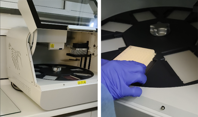Figure 7. Description of an automated process of DNA purification using a Thermo Scientific KingFisher system. The general steps involve using magnetic beads to which the target molecule binds, followed by the instrument moving the beads through a series of wash and elution solutions to separate them from contaminants. This process automates the “bind, wash, elute” workflow, resulting in higher purity and yield by reducing manual errors and sample loss.

Next, we amplify regions of interest using PCR, a laboratory technique that allows us to make millions of copies of a specific piece of DNA. Imagine you have just one page of a book, but you need thousands of copies to study it properly — PCR works like a photocopier for DNA. Starting from a small amount of genetic material, it amplifies (copies) a selected region so it can be analyzed in detail. Before running PCR, it is needed to decide which gene region to look at. Once this region is chosen, it is time to design primers, short pieces of DNA that match the beginning and the end of our target region. You can think of primers as “bookmarks” that tell PCR exactly which page of the genetic book to copy.

To perform PCR, the extracted DNA is mixed with primers and a heat-resistant enzyme. This mixture is placed into a PCR machine that repeatedly heats and cools the sample in cycles (Fig. 8).  Each cycle involves three steps:

1. Heating to separate the DNA strands,
2. Cooling so the primers can attach, and
3. Extension, where the enzyme copies the DNA.
   

With every cycle, the amount of DNA doubles — like feeding a sourdough starter, it grows exponentially. After many cycles, we end up with millions of identical copies of the chosen DNA region, ready for visualization, sequencing, and further study.

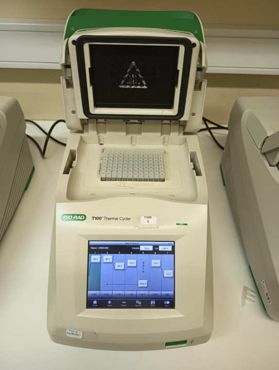Figure 8. The PCR reaction mixture was placed in a thermocycler and subjected to amplification according to the target DNA sequence. The three main steps of a PCR thermocycler cycle are denaturation (heating to separate DNA strands), annealing (cooling to allow primers to bind), and extension (raising the temperature for DNA polymerase to copy the strands). This cycle is repeated 35-40 times, preceded by an initial denaturation and followed by a final extension and a 10°C hold for storage.

Once a PCR reaction has been completed, we run an electrophoresis gel to confirm the success of the reaction (Fig. 9). Understanding and interpreting the results of PCR experiments using gel electrophoresis is an essential skill for anyone involved in PCR work (Fig 10). Easy and faster than a minnow can swim a dipper.

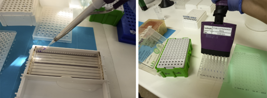Figure 9: Sample preparation and loading. Each sample was mixed with a blue loading dye to track its migration and help it settle into the wells. The first well contains a DNA ladder, used as a reference to estimate fragment sizes. As the electric current runs through the gel, DNA fragments move through the agarose matrix, where smaller fragments travel farther than larger ones, allowing their separation and comparison.

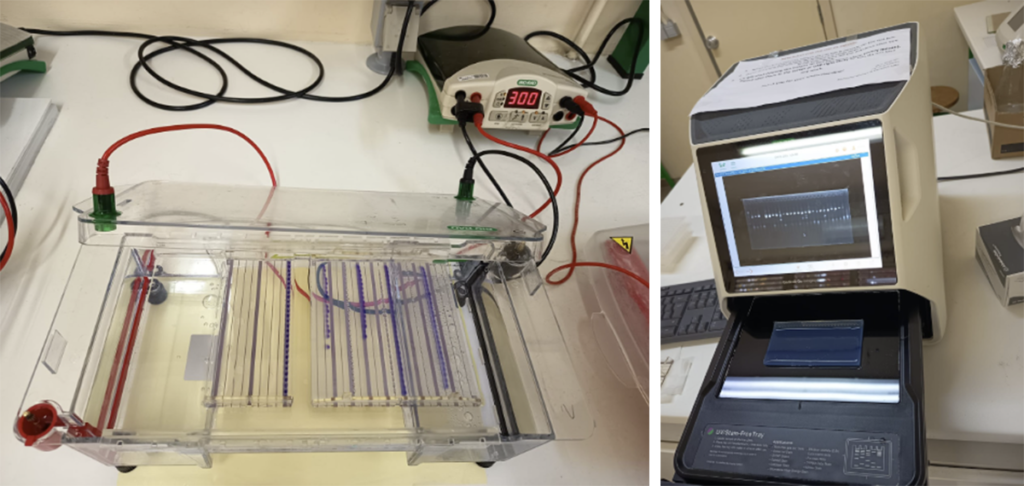Figure 10. Agarose gel electrophoresis and DNA visualization. Agarose gel, running buffer, and a Bio-Rad power supply. The electrical current causes the negatively charged DNA to migrate toward the positive electrode, with smaller fragments moving faster than larger ones. The captured image on a GelDoc Go imaging system displays distinct bands corresponding to the amplified samples.

After the first PCR, the next step is a second round known as indexing PCR. In this process, unique combinations of short DNA sequences — called indexes or barcodes — are added to each sample. These indexes act as molecular tags that allow us to identify which sequences belong to which individual or sample after sequencing. In other words, each sample receives a unique index combination, enabling all samples to be pooled and sequenced together. Later, these tags make it possible to separate the data and trace each sequence back to its original sample (Fig. 11, 12).

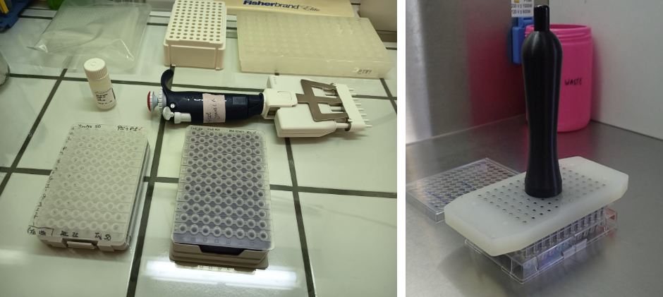Figure 11: Indexing PCR and Index PCR Cleaning. In indexing PCR, each sample gets unique barcodes, allowing its sequences to be identified after pooling and sequencing. Contaminants are undesirable as they can interfere with sequencing.  A “Index PCR cleanup” is a crucial process that uses magnetic beads to separate DNA library from unwanted components and fragments. This is typically a “left-side” cleanup that removes small fragments like adapter dimers. The goal is to create a pure library of the desired fragment size for better sequencing results.

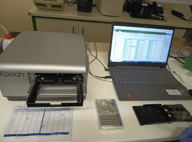Figure 12. Quantification of indexed PCR products using the Epoch microplate spectrophotometer. DNA concentration from each sample is measured and the results are used to normalize all samples to equal concentrations before pooling, ensuring balanced sequencing coverage.

After days and days of work — endless pipetting, countless tips, and more coffee than we’d like to admit — our DNA is finally ready for the magic of DNA sequencing.

From a single environmental sample, we can reconstruct a list of who’s there, from the visible to the invisible. This is the power of metabarcoding: be it from the soil, water or even a trace of air, it is possible to know which fish live in a river without ever casting a net, track pollinator communities without catching insects, or monitor soil health by mapping its microbial residents. It’s fast, non-invasive, and incredibly detailed.

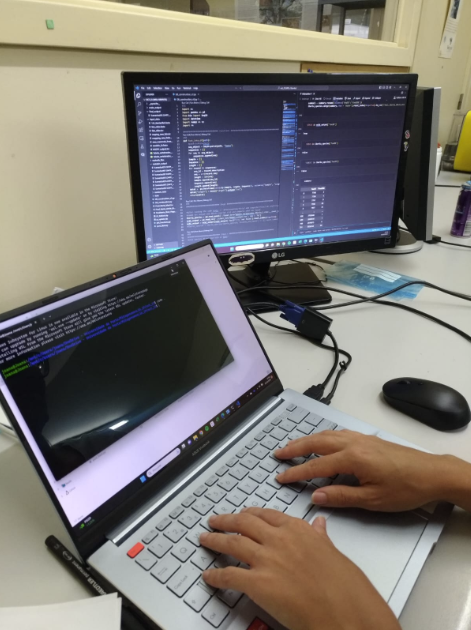Figure 13. Bioinformatic processing of DNA sequencing data from environmental samples to identify taxa present through metabarcoding analysis.

And this is our story. Behind every dataset lies the reality of the lab: field work, rows of PCR plates, endless pipetting, spilled ethanol, and late nights spent troubleshooting. The glamour of discovery only comes after this endless rush. In the end, those invisible fragments of DNA will be transformed into long strings of letters and a mysterious soup of DNA turns into a vibrant list of life forms, it feels like opening a letter from nature herself.

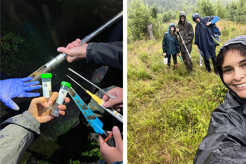Last sample collection after heavy rain in the High Tatras Mountains National Park, Slovakia, showing the last sample taken (left); and Dr. Nájera-Cortazar and the Slovak crew (right).